Bayesian Adaptive Sampling for Bayesian Model Averaging and Variable Selection in Linear Models
Source:R/bas_lm.R
bas.lm.RdSample without replacement from a posterior distribution on models
Usage
bas.lm(
  formula,
  data,
  subset,
  weights,
  contrasts = NULL,
  na.action = "na.omit",
  n.models = NULL,
  prior = "ZS-null",
  alpha = NULL,
  modelprior = beta.binomial(1, 1),
  initprobs = "Uniform",
  include.always = ~1,
  method = "BAS",
  update = NULL,
  bestmodel = NULL,
  prob.local = 0,
  prob.rw = 0.5,
  burnin.iterations = NULL,
  MCMC.iterations = NULL,
  lambda = NULL,
  delta = 0.025,
  thin = 1,
  renormalize = FALSE,
  importance.sampling = FALSE,
  FPS = "none",
  force.heredity = FALSE,
  pivot = TRUE,
  tol = 1e-07,
  GROW = TRUE,
  expand = 1.05,
  n.models.init = 2500,
  bigmem = FALSE
)
Arguments
- formula
linear model formula for the full model with all predictors, Y ~ X. All code assumes that an intercept will be included in each model and that the X's will be centered.
- data
a data frame. Factors will be converted to numerical vectors based on the using `model.matrix`.
- subset
an optional vector specifying a subset of observations to be used in the fitting process.
- weights
an optional vector of weights to be used in the fitting process. Should be NULL or a numeric vector. If non-NULL, Bayes estimates are obtained assuming that \(Y_i \sim N(x^T_i\beta, \sigma^2/w_i)\).
- contrasts
an optional list. See the contrasts.arg of `model.matrix.default()`.
- na.action
a function which indicates what should happen when the data contain NAs. The default is "na.omit".
- n.models
number of models to sample either without replacement (method="BAS" or "MCMC+BAS") or initial number of models to sample with replacement (method="MCMC" or "AMCMC"). If NULL,BAS with method="BAS" will try to enumerate/sample the min(2^p, 2^16). If 'n.models' > 2^25, the user should use 'bigmem = TRUE' to sample/enumerate 'n.models'. With method="MCMC" or "AMCMC", 'n.models' controls the initial number of models with the default for n.models = min(2000, 2^p). Sampling will stop once burnin.iterations + MCMC.iterations are exceeded and n.models will be increased/decreased as needed to store the unique models sampled. On exit 'n.models' is the number of unique models that have been sampled. For sampling with replacement (MCMC or AMCMC) the counts for the number of times a models is sampled is stored in the output as "freq".
- prior
prior distribution for regression coefficients. Choices include
"AIC"
"BIC"
"g-prior", Zellner's g prior where `g` is specified using the argument `alpha`
"JZS" Jeffreys-Zellner-Siow prior which uses the Jeffreys prior on sigma and the Zellner-Siow Cauchy prior on the coefficients. The optional parameter `alpha` can be used to control the squared scale of the prior, where the default is alpha=1. Setting `alpha` is equal to rscale^2 in the BayesFactor package of Morey. This uses QUADMATH for numerical integration of g.
"ZS-null", a Laplace approximation to the 'JZS' prior for integration of g. alpha = 1 only. We recommend using 'JZS' for accuracy and compatibility with the BayesFactor package, although it is slower.
"ZS-full" (to be deprecated)
"hyper-g", a mixture of g-priors where the prior on g/(1+g) is a Beta(1, alpha/2) as in Liang et al (2008). This uses the Cephes library for evaluation of the marginal likelihoods and may be numerically unstable for large n or R2 close to 1. Default choice of alpha is 3.
"hyper-g-laplace", Same as above but using a Laplace approximation to integrate over the prior on g.
"hyper-g-n", a mixture of g-priors that where u = g/n and u ~ Beta(1, alpha/2) to provide consistency when the null model is true.
"EB-local", use the MLE of g from the marginal likelihood within each model
"EB-global" uses an EM algorithm to find a common or global estimate of g, averaged over all models. When it is not possible to enumerate all models, the EM algorithm uses only the models sampled under EB-local.
- alpha
optional hyperparameter in g-prior or hyper g-prior. For Zellner's g-prior, alpha = g, for the Liang et al hyper-g or hyper-g-n method, recommended choice is alpha are between (2 < alpha < 4), with alpha = 3 the default. For the Zellner-Siow prior alpha = 1 by default, but can be used to modify the rate parameter in the gamma prior on g, $$1/g \sim G(1/2, n*\alpha/2)$$ so that $$\beta \sim C(0, \sigma^2 \alpha (X'X/n)^{-1})$$. If alpha = NULL, then the following defaults are used currently:
"g-prior" = n,
"hyper-g" = 3,
"EB-local" = 2,
"BIC" = n,
"ZS-null" = 1,
"ZS-full" = n,
"hyper-g-laplace" = 3,
"AIC" = 0,
"EB-global" = 2,
"hyper-g-n" = 3,
"JZS" = 1,
Note that Porwal & Raftery (2022) recommend alpha = sqrt(n) for the g-prior based on extensive range of simulations and examples for comparing BMA.
- modelprior
A function for a family of prior distribution on the models. Choices include
uniformBernoulliorbeta.binomial,tr.beta.binomial, (with truncation)tr.poisson(a truncated Poisson), andtr.power.prior(a truncated power family), with the default being abeta.binomial(1,1). Truncated versions are useful for p > n.- initprobs
Vector of length p or a character string specifying which method is used to create the vector. This is used to order variables for sampling all methods for potentially more efficient storage while sampling and provides the initial inclusion probabilities used for sampling without replacement with method="BAS". Options for the character string giving the method are: "Uniform" or "uniform" where each predictor variable is equally likely to be sampled (equivalent to random sampling without replacement); "eplogp" uses the
eplogprobfunction to approximate the Bayes factor from p-values from the full model to find initial marginal inclusion probabilities; "marg-eplogp" useseplogprob.margfunction to approximate the Bayes factor from p-values from the full model each simple linear regression. To run a Markov Chain to provide initial estimates of marginal inclusion probabilities for "BAS", use method="MCMC+BAS" below. While the initprobs are not used in sampling for method="MCMC", this determines the order of the variables in the lookup table and affects memory allocation in large problems where enumeration is not feasible. For variables that should always be included set the corresponding initprobs to 1, to override the `modelprior` or use `include.always` to force these variables to always be included in the model.- include.always
A formula with terms that should always be included in the model with probability one. By default this is `~ 1` meaning that the intercept is always included. This will also override any of the values in `initprobs` above by setting them to 1.
- method
A character variable indicating which sampling method to use:
"deterministic" uses the "top k" algorithm described in Ghosh and Clyde (2011) to sample models in order of approximate probability under conditional independence using the "initprobs". This is the most efficient algorithm for enumeration.
"BAS" uses Bayesian Adaptive Sampling (without replacement) using the sampling probabilities given in initprobs under a model of conditional independence. These can be updated based on estimates of the marginal inclusion probabilities.
"MCMC" samples with replacement via a MCMC algorithm that combines the birth/death random walk in Hoeting et al (1997) of MC3 with a random swap move to interchange a variable in the model with one currently excluded as described in Clyde, Ghosh and Littman (2010).
"MCMC+BAS" runs an initial MCMC to calculate marginal inclusion probabilities and then samples without replacement as in BAS. For BAS, the sampling probabilities can be updated as more models are sampled. (see update below).
"AMCMC" uses an adaptive proposal based on factoring the proposal distribution as a product conditional probabilities estimated from the past draws. If `importance.sampling = FALSE` this uses an adaptive independent Metropolis-Hasting algorithm, with if `importance.sampling = TRUE` uses importance sampling combined with Horwitz-Thompson estimates of posterior model and inclusion probabilities.
- update
number of iterations between potential updates of the sampling probabilities for method "BAS" or "MCMC+BAS". If NULL do not update, otherwise the algorithm will update using the marginal inclusion probabilities as they change while sampling takes place. For large model spaces, updating is recommended. If the model space will be enumerated, leave at the default.
- bestmodel
optional binary vector representing a model to initialize the sampling. If NULL sampling starts with the null model
- prob.local
A future option to allow sampling of models "near" the median probability model. Not used at this time.
- prob.rw
For any of the MCMC methods, probability of using the random-walk Metropolis proposal; otherwise use a random "flip" move to propose swap a variable that is excluded with a variable in the model.
- burnin.iterations
Number of burnin iterations for the MCMC sampler; the default is p*25 if not set by the user.
- MCMC.iterations
Number of iterations for the MCMC sampler; the default is p*1000 if not set by the user.
- lambda
Parameter in the AMCMC algorithm to insure positive definite covariance of gammas for adaptive conditional probabilities prior based on prior degrees of freedom pseudo in Inverse-Wishart. Default is set to p + 2.
- delta
truncation parameter to prevent sampling probabilities to degenerate to 0 or 1 prior to enumeration for sampling without replacement.
- thin
For "MCMC" or "MCMC+BAS", thin the MCMC chain every "thin" iterations; default is no thinning. For large p, thinning can be used to significantly reduce memory requirements as models and associated summaries are saved only every thin iterations. For thin = p, the model and associated output are recorded every p iterations, similar to the Gibbs sampler in SSVS.
- renormalize
For MCMC sampling, should posterior probabilities be based on renormalizing the marginal likelihoods times prior probabilities (TRUE) or frequencies from MCMC. The latter are unbiased in long runs, while the former may have less variability. May be compared via the diagnostic plot function
diagnostics. See details in Clyde and Ghosh (2012).- importance.sampling
whether to use importance sampling or an independent Metropolis-Hastings algorithm with sampling method="AMCMC" (see above).
- FPS
Finite Population Sampling estimator for use with method="MCMC+BAS". Options include "none" (default) which uses the sum of marginal likelihoods times priors for sampled models to estimate the normalizing constant, or "Bayes_HT" which uses an additional correction to the normalizing constant to account for unsampled models using sampling probabilities.
- force.heredity
Logical variable to force all levels of a factor to be included together and to include higher order interactions only if lower order terms are included. Currently supported with `method='MCMC'` and experimentally with `method='BAS'` on non-Solaris platforms. This is not compatible currently for enforcing hierachical constraints with orthogonal polynomials, poly(x, degree = 3). Without hereditary constraints the number of possible models with all possible interactions is 2^2^k where k is the number of factors with more than 2 levels. With hereditary constraints the number of models is much less, but computing this for k can be quite expensive for large k. For the model y ~ x1*x2*x3*x4*x5*x6) there are 7828353 models, which is more than 2^22. With n.models given, this will limit the number of models to the min(n.models, # models under the heredity constraints) Default is FALSE currently.
- pivot
Logical variable to allow pivoting of columns when obtaining the OLS estimates of a model so that models that are not full rank can be fit. Defaults to TRUE. Currently coefficients that are not estimable are set to zero. Use caution with interpreting BMA estimates of parameters.
- tol
1e-7 as
- GROW
Logical variable to indicate that the output vectors in MCMC are growable. Rather than allocate space based on `n.models`, the vectors will grow as needed if the number of unique models sampled exceeds the initial size of the allocated output vectors controlled by `n.models.init`. This is useful when `n.models` is unknown before reaching 'MCMC.iterations'. Default is TRUE.
- expand
variable to control how much to grow vectors with GROW = TRUE if number of unique models exceeds the current size of the vectors. The default is 1.25 times, which allows vectors to grow by 25 percent.
- n.models.init
Initial size of output vectors if GROW = TRUE. The default is `n.models = 2500`.
- bigmem
Logical variable to indicate that there is access to large amounts of memory (physical or virtual) for enumeration with large model spaces, e.g. > 2^25. default; used in determining rank of X^TX in Cholesky decomposition with pivoting.
Value
bas returns an object of class bas
An object of class BAS is a list containing at least the following
components:
- postprob
the posterior probabilities of the models selected
- priorprobs
the prior probabilities of the models selected
- namesx
the names of the variables
- R2
R2 values for the models
- logmarg
values of the log of the marginal likelihood for the models. This is equivalent to the log Bayes Factor for comparing each model to a base model with intercept only.
- n.vars
total number of independent variables in the full model, including the intercept
- size
the number of independent variables in each of the models, includes the intercept
- rank
the rank of the design matrix; if `pivot = FALSE`, this is the same as size as no checking of rank is conducted.
- which
a list of lists with one list per model with variables that are included in the model
- probne0
the posterior probability that each variable is non-zero computed using the renormalized marginal likelihoods of sampled models. This may be biased if the number of sampled models is much smaller than the total number of models. Unbiased estimates may be obtained using method "MCMC".
- mle
list of lists with one list per model giving the MLE (OLS) estimate of each (nonzero) coefficient for each model. NOTE: The intercept is the mean of Y as each column of X has been centered by subtracting its mean.
- mle.se
list of lists with one list per model giving the MLE (OLS) standard error of each coefficient for each model
- prior
the name of the prior that created the BMA object
- alpha
value of hyperparameter in coefficient prior used to create the BMA object.
- modelprior
the prior distribution on models that created the BMA object
- Y
response
- X
matrix of predictors
- mean.x
vector of means for each column of X (used in
predict.bas)- include.always
indices of variables that are forced into the model
The function summary.bas, is used to print a summary of the
results. The function plot.bas is used to plot posterior
distributions for the coefficients and image.bas provides an
image of the distribution over models. Posterior summaries of coefficients
can be extracted using coefficients.bas. Fitted values and
predictions can be obtained using the S3 functions fitted.bas
and predict.bas. BAS objects may be updated to use a
different prior (without rerunning the sampler) using the function
update.bas. For MCMC sampling diagnostics can be used
to assess whether the MCMC has run long enough so that the posterior probabilities
are stable. For more details see the associated demos and vignette.
Details
BAS provides several algorithms to sample from posterior distributions
of models for
use in Bayesian Model Averaging or Bayesian variable selection. For p less than
20-25, BAS can enumerate all models depending on memory availability. As BAS saves all
models, MLEs, standard errors, log marginal likelihoods, prior and posterior and probabilities
memory requirements grow linearly with M*p where M is the number of models
and p is the number of predictors. For example, enumeration with p=21 with 2,097,152 takes just under
2 Gigabytes on a 64 bit machine to store all summaries that would be needed for model averaging.
(A future version will likely include an option to not store all summaries if
users do not plan on using model averaging or model selection on Best Predictive models.)
For larger p, BAS samples without replacement using random or deterministic
sampling. The Bayesian Adaptive Sampling algorithm of Clyde, Ghosh, Littman
(2010) samples models without replacement using the initial sampling
probabilities, and will optionally update the sampling probabilities every
"update" models using the estimated marginal inclusion probabilities. BAS
uses different methods to obtain the initprobs, which may impact the
results in high-dimensional problems. The deterministic sampler provides a
list of the top models in order of an approximation of independence using
the provided initprobs. This may be effective after running the
other algorithms to identify high probability models and works well if the
correlations of variables are small to modest.
We recommend "MCMC" for
problems where enumeration is not feasible (memory or time constrained)
or even modest p if the number of
models sampled is not close to the number of possible models and/or there are significant
correlations among the predictors as the bias in estimates of inclusion
probabilities from "BAS" or "MCMC+BAS" may be large relative to the reduced
variability from using the normalized model probabilities as shown in Clyde and Ghosh, 2012.
Diagnostic plots with MCMC can be used to assess convergence.
For large problems we recommend thinning with MCMC to reduce memory requirements.
The priors on coefficients
include Zellner's g-prior, the Hyper-g prior (Liang et al 2008, the
Zellner-Siow Cauchy prior, Empirical Bayes (local and global) g-priors. AIC
and BIC are also included, while a range of priors on the model space are available.
References
Clyde, M. Ghosh, J. and Littman, M. (2010) Bayesian Adaptive
Sampling for Variable Selection and Model Averaging. Journal of
Computational Graphics and Statistics. 20:80-101
doi:10.1198/jcgs.2010.09049
Clyde, M. and Ghosh. J. (2012) Finite population estimators in stochastic search variable selection. Biometrika, 99 (4), 981-988. doi:10.1093/biomet/ass040
Clyde, M. and George, E. I. (2004) Model Uncertainty. Statist. Sci., 19,
81-94.
doi:10.1214/088342304000000035
Clyde, M. (1999) Bayesian Model Averaging and Model Search Strategies (with discussion). In Bayesian Statistics 6. J.M. Bernardo, A.P. Dawid, J.O. Berger, and A.F.M. Smith eds. Oxford University Press, pages 157-185.
Hoeting, J. A., Madigan, D., Raftery, A. E. and Volinsky, C. T. (1999)
Bayesian model averaging: a tutorial (with discussion). Statist. Sci., 14,
382-401.
doi:10.1214/ss/1009212519
Liang, F., Paulo, R., Molina, G., Clyde, M. and Berger, J.O. (2008) Mixtures
of g-priors for Bayesian Variable Selection. Journal of the American
Statistical Association. 103:410-423.
doi:10.1198/016214507000001337
Porwal, A. and Raftery, A. E. (2022) Comparing methods for statistical inference with model uncertainty PNAS 119 (16) e2120737119 doi:10.1073/pnas.2120737119
Zellner, A. (1986) On assessing prior distributions and Bayesian regression analysis with g-prior distributions. In Bayesian Inference and Decision Techniques: Essays in Honor of Bruno de Finetti, pp. 233-243. North-Holland/Elsevier.
Zellner, A. and Siow, A. (1980) Posterior odds ratios for selected regression hypotheses. In Bayesian Statistics: Proceedings of the First International Meeting held in Valencia (Spain), pp. 585-603.
Rouder, J. N., Speckman, P. L., Sun, D., Morey, R. D., and Iverson, G. (2009). Bayesian t-tests for accepting and rejecting the null hypothesis. Psychonomic Bulletin & Review, 16, 225-237
Rouder, J. N., Morey, R. D., Speckman, P. L., Province, J. M., (2012) Default Bayes Factors for ANOVA Designs. Journal of Mathematical Psychology. 56. p. 356-374.
See also
summary.bas, coefficients.bas,
print.bas, predict.bas, fitted.bas
plot.bas, image.bas, eplogprob,
update.bas
Other bas methods:
BAS,
coef.bas(),
confint.coef.bas(),
confint.pred.bas(),
diagnostics(),
fitted.bas(),
force.heredity.bas(),
image.bas(),
plot.confint.bas(),
predict.bas(),
predict.basglm(),
summary.bas(),
update.bas(),
variable.names.pred.bas()
Author
Merlise Clyde (clyde@duke.edu) and Michael Littman
Examples
library(MASS)
data(UScrime)
# pivot=FALSE is faster, but should only be used in full rank case
# default is pivot = TRUE
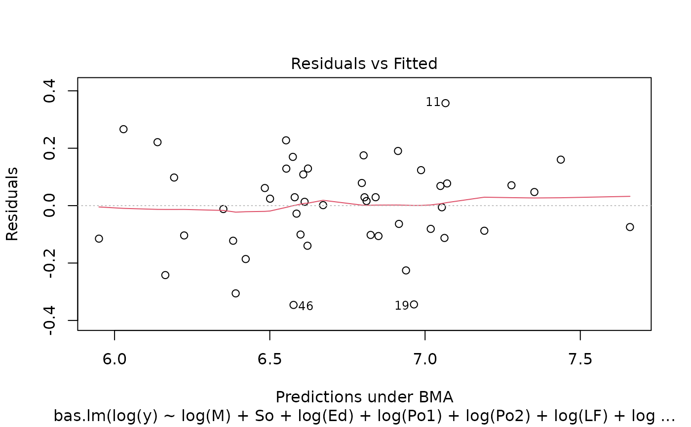
crime.bic <- bas.lm(log(y) ~ log(M) + So + log(Ed) +
log(Po1) + log(Po2) +
log(LF) + log(M.F) + log(Pop) + log(NW) +
log(U1) + log(U2) + log(GDP) + log(Ineq) +
log(Prob) + log(Time),
data = UScrime, n.models = 2^15, prior = "BIC",
modelprior = beta.binomial(1, 1),
initprobs = "eplogp", pivot = FALSE
)
# use MCMC rather than enumeration
crime.mcmc <- bas.lm(log(y) ~ log(M) + So + log(Ed) +
log(Po1) + log(Po2) +
log(LF) + log(M.F) + log(Pop) + log(NW) +
log(U1) + log(U2) + log(GDP) + log(Ineq) +
log(Prob) + log(Time),
data = UScrime,
method = "MCMC",
MCMC.iterations = 20000, prior = "BIC",
modelprior = beta.binomial(1, 1),
initprobs = "eplogp", pivot = FALSE
)
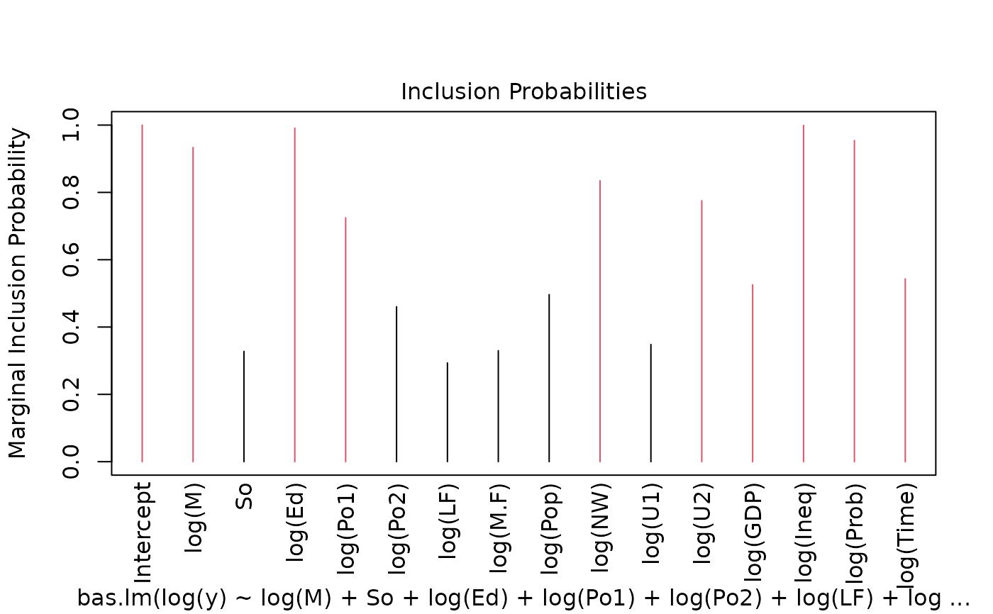
summary(crime.bic)
#> P(B != 0 | Y) model 1 model 2 model 3 model 4
#> Intercept 1.0000000 1.00000 1.000000e+00 1.0000000 1.0000000
#> log(M) 0.9335117 1.00000 1.000000e+00 1.0000000 1.0000000
#> So 0.3276563 0.00000 1.000000e+00 0.0000000 0.0000000
#> log(Ed) 0.9910219 1.00000 1.000000e+00 1.0000000 1.0000000
#> log(Po1) 0.7246635 1.00000 1.000000e+00 1.0000000 1.0000000
#> log(Po2) 0.4602481 0.00000 1.000000e+00 0.0000000 0.0000000
#> log(LF) 0.2935326 0.00000 1.000000e+00 0.0000000 0.0000000
#> log(M.F) 0.3298168 0.00000 1.000000e+00 0.0000000 0.0000000
#> log(Pop) 0.4962869 0.00000 1.000000e+00 0.0000000 0.0000000
#> log(NW) 0.8346412 1.00000 1.000000e+00 1.0000000 1.0000000
#> log(U1) 0.3481266 0.00000 1.000000e+00 0.0000000 0.0000000
#> log(U2) 0.7752102 1.00000 1.000000e+00 1.0000000 1.0000000
#> log(GDP) 0.5253694 0.00000 1.000000e+00 0.0000000 1.0000000
#> log(Ineq) 0.9992058 1.00000 1.000000e+00 1.0000000 1.0000000
#> log(Prob) 0.9541470 1.00000 1.000000e+00 1.0000000 1.0000000
#> log(Time) 0.5432686 1.00000 1.000000e+00 0.0000000 1.0000000
#> BF NA 1.00000 1.267935e-04 0.7609295 0.5431578
#> PostProbs NA 0.01910 1.560000e-02 0.0145000 0.0133000
#> R2 NA 0.84200 8.695000e-01 0.8265000 0.8506000
#> dim NA 9.00000 1.600000e+01 8.0000000 10.0000000
#> logmarg NA -22.15855 -3.113150e+01 -22.4317627 -22.7689035
#> model 5
#> Intercept 1.0000000
#> log(M) 1.0000000
#> So 0.0000000
#> log(Ed) 1.0000000
#> log(Po1) 1.0000000
#> log(Po2) 0.0000000
#> log(LF) 0.0000000
#> log(M.F) 0.0000000
#> log(Pop) 1.0000000
#> log(NW) 1.0000000
#> log(U1) 0.0000000
#> log(U2) 1.0000000
#> log(GDP) 0.0000000
#> log(Ineq) 1.0000000
#> log(Prob) 1.0000000
#> log(Time) 0.0000000
#> BF 0.5203179
#> PostProbs 0.0099000
#> R2 0.8375000
#> dim 9.0000000
#> logmarg -22.8118635
plot(crime.bic)


 image(crime.bic, subset = -1)
 # example with two-way interactions and hierarchical constraints
data(ToothGrowth)
ToothGrowth$dose <- factor(ToothGrowth$dose)
levels(ToothGrowth$dose) <- c("Low", "Medium", "High")
TG.bas <- bas.lm(len ~ supp * dose,
data = ToothGrowth,
modelprior = uniform(), method = "BAS",
force.heredity = TRUE
)
summary(TG.bas)
#> P(B != 0 | Y) model 1 model 2 model 3 model 4
#> Intercept 1.0000000 1.00000 1.0000000 1.00000000 1.000000e+00
#> suppVC 0.9910702 1.00000 1.0000000 0.00000000 0.000000e+00
#> doseMedium 1.0000000 1.00000 1.0000000 1.00000000 0.000000e+00
#> doseHigh 1.0000000 1.00000 1.0000000 1.00000000 0.000000e+00
#> suppVC:doseMedium 0.4500943 0.00000 1.0000000 0.00000000 0.000000e+00
#> suppVC:doseHigh 0.4500943 0.00000 1.0000000 0.00000000 0.000000e+00
#> BF NA 1.00000 0.8320043 0.01650685 2.812754e-15
#> PostProbs NA 0.54100 0.4501000 0.00890000 0.000000e+00
#> R2 NA 0.76230 0.7937000 0.70290000 0.000000e+00
#> dim NA 4.00000 6.0000000 3.00000000 1.000000e+00
#> logmarg NA 33.50461 33.3206946 29.40063248 0.000000e+00
#> model 5
#> Intercept 1.000000e+00
#> suppVC 1.000000e+00
#> doseMedium 0.000000e+00
#> doseHigh 0.000000e+00
#> suppVC:doseMedium 0.000000e+00
#> suppVC:doseHigh 0.000000e+00
#> BF 7.895214e-16
#> PostProbs 0.000000e+00
#> R2 5.950000e-02
#> dim 2.000000e+00
#> logmarg -1.270492e+00
image(TG.bas)
# example with two-way interactions and hierarchical constraints
data(ToothGrowth)
ToothGrowth$dose <- factor(ToothGrowth$dose)
levels(ToothGrowth$dose) <- c("Low", "Medium", "High")
TG.bas <- bas.lm(len ~ supp * dose,
data = ToothGrowth,
modelprior = uniform(), method = "BAS",
force.heredity = TRUE
)
summary(TG.bas)
#> P(B != 0 | Y) model 1 model 2 model 3 model 4
#> Intercept 1.0000000 1.00000 1.0000000 1.00000000 1.000000e+00
#> suppVC 0.9910702 1.00000 1.0000000 0.00000000 0.000000e+00
#> doseMedium 1.0000000 1.00000 1.0000000 1.00000000 0.000000e+00
#> doseHigh 1.0000000 1.00000 1.0000000 1.00000000 0.000000e+00
#> suppVC:doseMedium 0.4500943 0.00000 1.0000000 0.00000000 0.000000e+00
#> suppVC:doseHigh 0.4500943 0.00000 1.0000000 0.00000000 0.000000e+00
#> BF NA 1.00000 0.8320043 0.01650685 2.812754e-15
#> PostProbs NA 0.54100 0.4501000 0.00890000 0.000000e+00
#> R2 NA 0.76230 0.7937000 0.70290000 0.000000e+00
#> dim NA 4.00000 6.0000000 3.00000000 1.000000e+00
#> logmarg NA 33.50461 33.3206946 29.40063248 0.000000e+00
#> model 5
#> Intercept 1.000000e+00
#> suppVC 1.000000e+00
#> doseMedium 0.000000e+00
#> doseHigh 0.000000e+00
#> suppVC:doseMedium 0.000000e+00
#> suppVC:doseHigh 0.000000e+00
#> BF 7.895214e-16
#> PostProbs 0.000000e+00
#> R2 5.950000e-02
#> dim 2.000000e+00
#> logmarg -1.270492e+00
image(TG.bas)
 # don't run the following due to time limits on CRAN
if (FALSE) { # \dontrun{
# exmple with non-full rank case
loc <- system.file("testdata", package = "BAS")
d <- read.csv(paste(loc, "JASP-testdata.csv", sep = "/"))
fullModelFormula <- as.formula("contNormal ~ contGamma * contExpon +
contGamma * contcor1 + contExpon * contcor1")
# should trigger a warning (default is to use pivoting, so use pivot=FALSE
# only for full rank case)
out = bas.lm(fullModelFormula,
data = d,
alpha = 0.125316,
prior = "JZS",
weights = facFifty, force.heredity = FALSE, pivot = FALSE)
# use pivot = TRUE to fit non-full rank case (default)
# This is slower but safer
out = bas.lm(fullModelFormula,
data = d,
alpha = 0.125316,
prior = "JZS",
weights = facFifty, force.heredity = FALSE, pivot = TRUE)
} # }
# more complete demo's
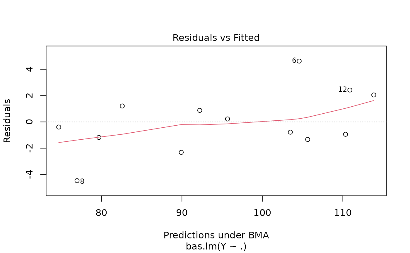
demo(BAS.hald)
#>
#>
#> demo(BAS.hald)
#> ---- ~~~~~~~~
#>
#> > data(Hald)
#>
#> > hald.gprior = bas.lm(Y~ ., data=Hald, prior="g-prior", alpha=13,
#> + modelprior=beta.binomial(1,1),
#> + initprobs="eplogp")
#>
#> > hald.gprior
#>
#> Call:
#> bas.lm(formula = Y ~ ., data = Hald, prior = "g-prior", alpha = 13,
#> modelprior = beta.binomial(1, 1), initprobs = "eplogp")
#>
#>
#> Marginal Posterior Inclusion Probabilities:
#> Intercept X1 X2 X3 X4
#> 1.0000 0.9019 0.6896 0.4653 0.6329
#>
#> > plot(hald.gprior)
# don't run the following due to time limits on CRAN
if (FALSE) { # \dontrun{
# exmple with non-full rank case
loc <- system.file("testdata", package = "BAS")
d <- read.csv(paste(loc, "JASP-testdata.csv", sep = "/"))
fullModelFormula <- as.formula("contNormal ~ contGamma * contExpon +
contGamma * contcor1 + contExpon * contcor1")
# should trigger a warning (default is to use pivoting, so use pivot=FALSE
# only for full rank case)
out = bas.lm(fullModelFormula,
data = d,
alpha = 0.125316,
prior = "JZS",
weights = facFifty, force.heredity = FALSE, pivot = FALSE)
# use pivot = TRUE to fit non-full rank case (default)
# This is slower but safer
out = bas.lm(fullModelFormula,
data = d,
alpha = 0.125316,
prior = "JZS",
weights = facFifty, force.heredity = FALSE, pivot = TRUE)
} # }
# more complete demo's
demo(BAS.hald)
#>
#>
#> demo(BAS.hald)
#> ---- ~~~~~~~~
#>
#> > data(Hald)
#>
#> > hald.gprior = bas.lm(Y~ ., data=Hald, prior="g-prior", alpha=13,
#> + modelprior=beta.binomial(1,1),
#> + initprobs="eplogp")
#>
#> > hald.gprior
#>
#> Call:
#> bas.lm(formula = Y ~ ., data = Hald, prior = "g-prior", alpha = 13,
#> modelprior = beta.binomial(1, 1), initprobs = "eplogp")
#>
#>
#> Marginal Posterior Inclusion Probabilities:
#> Intercept X1 X2 X3 X4
#> 1.0000 0.9019 0.6896 0.4653 0.6329
#>
#> > plot(hald.gprior)


 #>
#> > summary(hald.gprior)
#> P(B != 0 | Y) model 1 model 2 model 3 model 4 model 5
#> Intercept 1.0000000 1.00000 1.0000000 1.00000000 1.0000000 1.0000000
#> X1 0.9019245 1.00000 1.0000000 1.00000000 1.0000000 1.0000000
#> X2 0.6895830 1.00000 0.0000000 1.00000000 1.0000000 1.0000000
#> X3 0.4652762 0.00000 0.0000000 1.00000000 0.0000000 1.0000000
#> X4 0.6329266 0.00000 1.0000000 1.00000000 1.0000000 0.0000000
#> BF NA 1.00000 0.6923944 0.08991408 0.3355714 0.3344926
#> PostProbs NA 0.24320 0.1684000 0.13120000 0.1224000 0.1220000
#> R2 NA 0.97870 0.9725000 0.98240000 0.9823000 0.9823000
#> dim NA 3.00000 3.0000000 5.00000000 4.0000000 4.0000000
#> logmarg NA 11.72735 11.3597547 9.31845348 10.6354335 10.6322138
#>
#> > image(hald.gprior, subset=-1, vlas=0)
#>
#> > summary(hald.gprior)
#> P(B != 0 | Y) model 1 model 2 model 3 model 4 model 5
#> Intercept 1.0000000 1.00000 1.0000000 1.00000000 1.0000000 1.0000000
#> X1 0.9019245 1.00000 1.0000000 1.00000000 1.0000000 1.0000000
#> X2 0.6895830 1.00000 0.0000000 1.00000000 1.0000000 1.0000000
#> X3 0.4652762 0.00000 0.0000000 1.00000000 0.0000000 1.0000000
#> X4 0.6329266 0.00000 1.0000000 1.00000000 1.0000000 0.0000000
#> BF NA 1.00000 0.6923944 0.08991408 0.3355714 0.3344926
#> PostProbs NA 0.24320 0.1684000 0.13120000 0.1224000 0.1220000
#> R2 NA 0.97870 0.9725000 0.98240000 0.9823000 0.9823000
#> dim NA 3.00000 3.0000000 5.00000000 4.0000000 4.0000000
#> logmarg NA 11.72735 11.3597547 9.31845348 10.6354335 10.6322138
#>
#> > image(hald.gprior, subset=-1, vlas=0)
 #>
#> > hald.coef = coefficients(hald.gprior)
#>
#> > hald.coef
#>
#> Marginal Posterior Summaries of Coefficients:
#>
#> Using BMA
#>
#> Based on the top 16 models
#> post mean post SD post p(B != 0)
#> Intercept 95.4231 0.7107 1.0000
#> X1 1.2150 0.5190 0.9019
#> X2 0.2756 0.4832 0.6896
#> X3 -0.1271 0.4976 0.4653
#> X4 -0.3269 0.4717 0.6329
#>
#> > plot(hald.coef)
#>
#> > hald.coef = coefficients(hald.gprior)
#>
#> > hald.coef
#>
#> Marginal Posterior Summaries of Coefficients:
#>
#> Using BMA
#>
#> Based on the top 16 models
#> post mean post SD post p(B != 0)
#> Intercept 95.4231 0.7107 1.0000
#> X1 1.2150 0.5190 0.9019
#> X2 0.2756 0.4832 0.6896
#> X3 -0.1271 0.4976 0.4653
#> X4 -0.3269 0.4717 0.6329
#>
#> > plot(hald.coef)


 #>
#> > predict(hald.gprior, top=5, se.fit=TRUE)
#> $fit
#> [1] 79.74246 74.50010 105.29268 89.88693 95.57177 104.56409 103.40145
#> [8] 77.13668 91.99731 114.21325 82.78446 111.00723 110.40160
#>
#> $Ybma
#> [,1]
#> [1,] 79.74246
#> [2,] 74.50010
#> [3,] 105.29268
#> [4,] 89.88693
#> [5,] 95.57177
#> [6,] 104.56409
#> [7,] 103.40145
#> [8,] 77.13668
#> [9,] 91.99731
#> [10,] 114.21325
#> [11,] 82.78446
#> [12,] 111.00723
#> [13,] 110.40160
#>
#> $Ypred
#> [,1] [,2] [,3] [,4] [,5] [,6] [,7] [,8]
#> [1,] 81.17036 74.83464 105.0725 89.69881 97.15898 104.4575 103.3893 76.06454
#> [2,] 77.70296 74.24113 105.8554 90.46267 93.09565 104.7152 103.1399 78.80193
#> [3,] 79.70437 74.40553 105.2175 89.76253 95.63309 104.5709 103.5254 77.08557
#> [4,] 79.65151 74.47846 105.4218 89.83174 95.62799 104.5962 103.5068 77.00839
#> [5,] 79.84321 74.31409 104.9063 89.65651 95.70301 104.5285 103.5476 77.15919
#> [,9] [,10] [,11] [,12] [,13]
#> [1,] 91.57174 113.1722 81.59906 111.2219 111.0884
#> [2,] 92.68123 115.8058 84.50293 110.4162 109.0791
#> [3,] 91.98604 114.1759 82.78145 111.1196 110.5321
#> [4,] 92.07571 114.1088 82.68233 111.0429 110.4674
#> [5,] 91.83513 114.2353 82.88128 111.2384 110.6515
#>
#> $postprobs
#> [1] 0.3089304 0.2139017 0.1666632 0.1555023 0.1550024
#>
#> $se.fit
#> [,1] [,2] [,3] [,4] [,5] [,6] [,7] [,8]
#> [1,] 2.220164 2.265862 1.546911 2.181188 1.310135 1.523300 2.655096 2.176560
#> [2,] 2.716798 2.389723 1.633637 2.179215 1.321062 1.581232 2.721957 2.078129
#> [3,] 3.203405 2.501485 3.279273 2.357164 2.589756 1.549136 2.623290 2.765255
#> [4,] 3.117350 2.283957 1.602160 2.149087 2.589321 1.508471 2.610923 2.545817
#> [5,] 2.932580 2.353352 1.538009 2.141694 2.507848 1.498758 2.616407 2.680289
#> [,9] [,10] [,11] [,12] [,13]
#> [1,] 1.883610 3.264656 1.908238 1.970691 2.054234
#> [2,] 2.013244 3.298134 1.933819 1.964374 1.924460
#> [3,] 2.353516 3.609909 2.821295 2.227363 2.390135
#> [4,] 1.990817 3.485929 2.456636 1.951456 2.212238
#> [5,] 1.889302 3.569065 2.665166 1.934336 2.117189
#>
#> $se.pred
#> [,1] [,2] [,3] [,4] [,5] [,6] [,7] [,8]
#> [1,] 5.057182 5.077410 4.799885 5.040193 4.728892 4.792328 5.262651 5.038191
#> [2,] 5.415848 5.259391 4.961773 5.167146 4.867815 4.944766 5.418438 5.125333
#> [3,] 5.489152 5.111401 5.533771 5.042342 5.155175 4.718984 5.172102 5.245534
#> [4,] 5.440156 5.009380 4.737547 4.949344 5.155775 4.706689 5.166658 5.134065
#> [5,] 5.337427 5.042456 4.717369 4.947217 5.116386 4.704719 5.170463 5.203081
#> [,9] [,10] [,11] [,12] [,13]
#> [1,] 4.918734 5.594992 4.928218 4.952735 4.986566
#> [2,] 5.099370 5.729582 5.068538 5.080274 5.064974
#> [3,] 5.040638 5.735890 5.275291 4.982985 5.057839
#> [4,] 4.882702 5.659428 5.090431 4.866787 4.977090
#> [5,] 4.843301 5.711946 5.195307 4.861045 4.936658
#>
#> $se.bma.fit
#> [1] 2.688224 2.095245 1.769625 1.970919 2.197285 1.363804 2.356457 2.302631
#> [9] 1.822084 3.141443 2.237663 1.801849 1.991374
#>
#> $se.bma.pred
#> [1] 4.838655 4.536087 4.395180 4.480017 4.584113 4.248058 4.662502 4.635531
#> [9] 4.416563 5.104380 4.603604 4.408253 4.489054
#>
#> $df
#> [1] 12 12 12 12 12
#>
#> $best
#> [1] 12 4 8 9 5
#>
#> $bestmodel
#> $bestmodel[[1]]
#> [1] 0 1 2
#>
#> $bestmodel[[2]]
#> [1] 0 1 4
#>
#> $bestmodel[[3]]
#> [1] 0 1 2 3 4
#>
#> $bestmodel[[4]]
#> [1] 0 1 2 4
#>
#> $bestmodel[[5]]
#> [1] 0 1 2 3
#>
#>
#> $best.vars
#> [1] "Intercept" "X1" "X2" "X3" "X4"
#>
#> $estimator
#> [1] "BMA"
#>
#> attr(,"class")
#> [1] "pred.bas"
#>
#> > confint(predict(hald.gprior, Hald, estimator="BMA", se.fit=TRUE, top=5), parm="mean")
#> 2.5% 97.5% mean
#> [1,] 73.04460 85.99670 79.74246
#> [2,] 69.08615 79.45953 74.50010
#> [3,] 100.86586 109.45991 105.29268
#> [4,] 85.00337 94.63284 89.88693
#> [5,] 90.49220 100.57608 95.57177
#> [6,] 101.17646 107.81954 104.56409
#> [7,] 97.63097 109.15498 103.40145
#> [8,] 71.68036 82.81063 77.13668
#> [9,] 87.34153 96.32155 91.99731
#> [10,] 106.67199 122.05730 114.21325
#> [11,] 77.41298 88.04204 82.78446
#> [12,] 106.75325 115.55596 111.00723
#> [13,] 105.46200 115.14501 110.40160
#> attr(,"Probability")
#> [1] 0.95
#> attr(,"class")
#> [1] "confint.bas"
#>
#> > predict(hald.gprior, estimator="MPM", se.fit=TRUE)
#> $fit
#> [1] 79.65151 74.47846 105.42183 89.83174 95.62799 104.59616 103.50684
#> [8] 77.00839 92.07571 114.10876 82.68233 111.04286 110.46741
#> attr(,"model")
#> [1] 0 1 2 4
#> attr(,"best")
#> [1] 1
#> attr(,"estimator")
#> [1] "MPM"
#>
#> $Ybma
#> [1] 79.65151 74.47846 105.42183 89.83174 95.62799 104.59616 103.50684
#> [8] 77.00839 92.07571 114.10876 82.68233 111.04286 110.46741
#> attr(,"model")
#> [1] 0 1 2 4
#> attr(,"best")
#> [1] 1
#> attr(,"estimator")
#> [1] "MPM"
#>
#> $Ypred
#> NULL
#>
#> $postprobs
#> NULL
#>
#> $se.fit
#> [1] 3.117350 2.283957 1.602160 2.149087 2.589321 1.508471 2.610923 2.545817
#> [9] 1.990817 3.485929 2.456636 1.951456 2.212238
#>
#> $se.pred
#> [1] 5.440156 5.009380 4.737547 4.949344 5.155775 4.706689 5.166658 5.134065
#> [9] 4.882702 5.659428 5.090431 4.866787 4.977090
#>
#> $se.bma.fit
#> NULL
#>
#> $se.bma.pred
#> NULL
#>
#> $df
#> [1] 12
#>
#> $best
#> NULL
#>
#> $bestmodel
#> [1] 0 1 2 4
#>
#> $best.vars
#> [1] "Intercept" "X1" "X2" "X4"
#>
#> $estimator
#> [1] "MPM"
#>
#> attr(,"class")
#> [1] "pred.bas"
#>
#> > confint(predict(hald.gprior, Hald, estimator="MPM", se.fit=TRUE), parm="mean")
#> 2.5% 97.5% mean
#> [1,] 72.85939 86.44363 79.65151
#> [2,] 69.50215 79.45478 74.47846
#> [3,] 101.93102 108.91264 105.42183
#> [4,] 85.14928 94.51420 89.83174
#> [5,] 89.98634 101.26964 95.62799
#> [6,] 101.30948 107.88283 104.59616
#> [7,] 97.81813 109.19556 103.50684
#> [8,] 71.46153 82.55525 77.00839
#> [9,] 87.73810 96.41333 92.07571
#> [10,] 106.51357 121.70394 114.10876
#> [11,] 77.32978 88.03488 82.68233
#> [12,] 106.79101 115.29472 111.04286
#> [13,] 105.64736 115.28746 110.46741
#> attr(,"Probability")
#> [1] 0.95
#> attr(,"class")
#> [1] "confint.bas"
#>
#> > fitted(hald.gprior, estimator="HPM")
#> [1] 81.17036 74.83464 105.07248 89.69881 97.15898 104.45753 103.38927
#> [8] 76.06454 91.57174 113.17222 81.59906 111.22195 111.08841
#>
#> > hald.gprior = bas.lm(Y~ ., data=Hald, n.models=2^4,
#> + prior="g-prior", alpha=13, modelprior=uniform(),
#> + initprobs="eplogp")
#>
#> > hald.EB = update(hald.gprior, newprior="EB-global")
#>
#> > hald.bic = update(hald.gprior,newprior="BIC")
#>
#> > hald.zs = update(hald.bic, newprior="ZS-null")
if (FALSE) { # \dontrun{
demo(BAS.USCrime)
} # }
#>
#> > predict(hald.gprior, top=5, se.fit=TRUE)
#> $fit
#> [1] 79.74246 74.50010 105.29268 89.88693 95.57177 104.56409 103.40145
#> [8] 77.13668 91.99731 114.21325 82.78446 111.00723 110.40160
#>
#> $Ybma
#> [,1]
#> [1,] 79.74246
#> [2,] 74.50010
#> [3,] 105.29268
#> [4,] 89.88693
#> [5,] 95.57177
#> [6,] 104.56409
#> [7,] 103.40145
#> [8,] 77.13668
#> [9,] 91.99731
#> [10,] 114.21325
#> [11,] 82.78446
#> [12,] 111.00723
#> [13,] 110.40160
#>
#> $Ypred
#> [,1] [,2] [,3] [,4] [,5] [,6] [,7] [,8]
#> [1,] 81.17036 74.83464 105.0725 89.69881 97.15898 104.4575 103.3893 76.06454
#> [2,] 77.70296 74.24113 105.8554 90.46267 93.09565 104.7152 103.1399 78.80193
#> [3,] 79.70437 74.40553 105.2175 89.76253 95.63309 104.5709 103.5254 77.08557
#> [4,] 79.65151 74.47846 105.4218 89.83174 95.62799 104.5962 103.5068 77.00839
#> [5,] 79.84321 74.31409 104.9063 89.65651 95.70301 104.5285 103.5476 77.15919
#> [,9] [,10] [,11] [,12] [,13]
#> [1,] 91.57174 113.1722 81.59906 111.2219 111.0884
#> [2,] 92.68123 115.8058 84.50293 110.4162 109.0791
#> [3,] 91.98604 114.1759 82.78145 111.1196 110.5321
#> [4,] 92.07571 114.1088 82.68233 111.0429 110.4674
#> [5,] 91.83513 114.2353 82.88128 111.2384 110.6515
#>
#> $postprobs
#> [1] 0.3089304 0.2139017 0.1666632 0.1555023 0.1550024
#>
#> $se.fit
#> [,1] [,2] [,3] [,4] [,5] [,6] [,7] [,8]
#> [1,] 2.220164 2.265862 1.546911 2.181188 1.310135 1.523300 2.655096 2.176560
#> [2,] 2.716798 2.389723 1.633637 2.179215 1.321062 1.581232 2.721957 2.078129
#> [3,] 3.203405 2.501485 3.279273 2.357164 2.589756 1.549136 2.623290 2.765255
#> [4,] 3.117350 2.283957 1.602160 2.149087 2.589321 1.508471 2.610923 2.545817
#> [5,] 2.932580 2.353352 1.538009 2.141694 2.507848 1.498758 2.616407 2.680289
#> [,9] [,10] [,11] [,12] [,13]
#> [1,] 1.883610 3.264656 1.908238 1.970691 2.054234
#> [2,] 2.013244 3.298134 1.933819 1.964374 1.924460
#> [3,] 2.353516 3.609909 2.821295 2.227363 2.390135
#> [4,] 1.990817 3.485929 2.456636 1.951456 2.212238
#> [5,] 1.889302 3.569065 2.665166 1.934336 2.117189
#>
#> $se.pred
#> [,1] [,2] [,3] [,4] [,5] [,6] [,7] [,8]
#> [1,] 5.057182 5.077410 4.799885 5.040193 4.728892 4.792328 5.262651 5.038191
#> [2,] 5.415848 5.259391 4.961773 5.167146 4.867815 4.944766 5.418438 5.125333
#> [3,] 5.489152 5.111401 5.533771 5.042342 5.155175 4.718984 5.172102 5.245534
#> [4,] 5.440156 5.009380 4.737547 4.949344 5.155775 4.706689 5.166658 5.134065
#> [5,] 5.337427 5.042456 4.717369 4.947217 5.116386 4.704719 5.170463 5.203081
#> [,9] [,10] [,11] [,12] [,13]
#> [1,] 4.918734 5.594992 4.928218 4.952735 4.986566
#> [2,] 5.099370 5.729582 5.068538 5.080274 5.064974
#> [3,] 5.040638 5.735890 5.275291 4.982985 5.057839
#> [4,] 4.882702 5.659428 5.090431 4.866787 4.977090
#> [5,] 4.843301 5.711946 5.195307 4.861045 4.936658
#>
#> $se.bma.fit
#> [1] 2.688224 2.095245 1.769625 1.970919 2.197285 1.363804 2.356457 2.302631
#> [9] 1.822084 3.141443 2.237663 1.801849 1.991374
#>
#> $se.bma.pred
#> [1] 4.838655 4.536087 4.395180 4.480017 4.584113 4.248058 4.662502 4.635531
#> [9] 4.416563 5.104380 4.603604 4.408253 4.489054
#>
#> $df
#> [1] 12 12 12 12 12
#>
#> $best
#> [1] 12 4 8 9 5
#>
#> $bestmodel
#> $bestmodel[[1]]
#> [1] 0 1 2
#>
#> $bestmodel[[2]]
#> [1] 0 1 4
#>
#> $bestmodel[[3]]
#> [1] 0 1 2 3 4
#>
#> $bestmodel[[4]]
#> [1] 0 1 2 4
#>
#> $bestmodel[[5]]
#> [1] 0 1 2 3
#>
#>
#> $best.vars
#> [1] "Intercept" "X1" "X2" "X3" "X4"
#>
#> $estimator
#> [1] "BMA"
#>
#> attr(,"class")
#> [1] "pred.bas"
#>
#> > confint(predict(hald.gprior, Hald, estimator="BMA", se.fit=TRUE, top=5), parm="mean")
#> 2.5% 97.5% mean
#> [1,] 73.04460 85.99670 79.74246
#> [2,] 69.08615 79.45953 74.50010
#> [3,] 100.86586 109.45991 105.29268
#> [4,] 85.00337 94.63284 89.88693
#> [5,] 90.49220 100.57608 95.57177
#> [6,] 101.17646 107.81954 104.56409
#> [7,] 97.63097 109.15498 103.40145
#> [8,] 71.68036 82.81063 77.13668
#> [9,] 87.34153 96.32155 91.99731
#> [10,] 106.67199 122.05730 114.21325
#> [11,] 77.41298 88.04204 82.78446
#> [12,] 106.75325 115.55596 111.00723
#> [13,] 105.46200 115.14501 110.40160
#> attr(,"Probability")
#> [1] 0.95
#> attr(,"class")
#> [1] "confint.bas"
#>
#> > predict(hald.gprior, estimator="MPM", se.fit=TRUE)
#> $fit
#> [1] 79.65151 74.47846 105.42183 89.83174 95.62799 104.59616 103.50684
#> [8] 77.00839 92.07571 114.10876 82.68233 111.04286 110.46741
#> attr(,"model")
#> [1] 0 1 2 4
#> attr(,"best")
#> [1] 1
#> attr(,"estimator")
#> [1] "MPM"
#>
#> $Ybma
#> [1] 79.65151 74.47846 105.42183 89.83174 95.62799 104.59616 103.50684
#> [8] 77.00839 92.07571 114.10876 82.68233 111.04286 110.46741
#> attr(,"model")
#> [1] 0 1 2 4
#> attr(,"best")
#> [1] 1
#> attr(,"estimator")
#> [1] "MPM"
#>
#> $Ypred
#> NULL
#>
#> $postprobs
#> NULL
#>
#> $se.fit
#> [1] 3.117350 2.283957 1.602160 2.149087 2.589321 1.508471 2.610923 2.545817
#> [9] 1.990817 3.485929 2.456636 1.951456 2.212238
#>
#> $se.pred
#> [1] 5.440156 5.009380 4.737547 4.949344 5.155775 4.706689 5.166658 5.134065
#> [9] 4.882702 5.659428 5.090431 4.866787 4.977090
#>
#> $se.bma.fit
#> NULL
#>
#> $se.bma.pred
#> NULL
#>
#> $df
#> [1] 12
#>
#> $best
#> NULL
#>
#> $bestmodel
#> [1] 0 1 2 4
#>
#> $best.vars
#> [1] "Intercept" "X1" "X2" "X4"
#>
#> $estimator
#> [1] "MPM"
#>
#> attr(,"class")
#> [1] "pred.bas"
#>
#> > confint(predict(hald.gprior, Hald, estimator="MPM", se.fit=TRUE), parm="mean")
#> 2.5% 97.5% mean
#> [1,] 72.85939 86.44363 79.65151
#> [2,] 69.50215 79.45478 74.47846
#> [3,] 101.93102 108.91264 105.42183
#> [4,] 85.14928 94.51420 89.83174
#> [5,] 89.98634 101.26964 95.62799
#> [6,] 101.30948 107.88283 104.59616
#> [7,] 97.81813 109.19556 103.50684
#> [8,] 71.46153 82.55525 77.00839
#> [9,] 87.73810 96.41333 92.07571
#> [10,] 106.51357 121.70394 114.10876
#> [11,] 77.32978 88.03488 82.68233
#> [12,] 106.79101 115.29472 111.04286
#> [13,] 105.64736 115.28746 110.46741
#> attr(,"Probability")
#> [1] 0.95
#> attr(,"class")
#> [1] "confint.bas"
#>
#> > fitted(hald.gprior, estimator="HPM")
#> [1] 81.17036 74.83464 105.07248 89.69881 97.15898 104.45753 103.38927
#> [8] 76.06454 91.57174 113.17222 81.59906 111.22195 111.08841
#>
#> > hald.gprior = bas.lm(Y~ ., data=Hald, n.models=2^4,
#> + prior="g-prior", alpha=13, modelprior=uniform(),
#> + initprobs="eplogp")
#>
#> > hald.EB = update(hald.gprior, newprior="EB-global")
#>
#> > hald.bic = update(hald.gprior,newprior="BIC")
#>
#> > hald.zs = update(hald.bic, newprior="ZS-null")
if (FALSE) { # \dontrun{
demo(BAS.USCrime)
} # }