Nonparametric Regression with Bayesian Additive Regression Kernels
Merlise A Clyde
2024-10-06
Source:vignettes/bark.Rmd
bark.RmdBayesian Additive Regression Kernel (BARK) models are a flexible Bayesian nonparametric model for regression and classification problems where the unknown mean function is represented as a weighted sum of multivariate Gaussian kernel functions, that allows nonlinearities, interactions and feature selection using Levy random fields to construct a prior on the unknown function. Each kernel is centered at location parameters with precision parameters - these precision parameters capture the importance of each of the dimensional predictor variables and by setting a to zero may remove important variables that are not important.
Installation
To get the latest version of {r bark}, install from github (needs compilation))
devtools::install_github("merliseclyde/bark")Example
We will illustrate feature selection in a simple simulated example from Friedman
set.seed(42)
traindata <- data.frame(sim_Friedman2(200, sd=125))
testdata <- data.frame(sim_Friedman2(1000, sd=0))
set.seed(42)
fit.bark.d <- bark(y ~ ., data = traindata,
                   testdata= testdata,
                   classification=FALSE,
                   selection = FALSE,
                   common_lambdas = FALSE,
#                   fixed = list(eps = .25, gam = 2.5),
                   nburn = 100,
                   nkeep = 250,
                   printevery = 10^10)

mean((fit.bark.d$yhat.test.mean-testdata$y)^2)
#> [1] 1604.15
set.seed(42)
fit.bark.sd <- bark(y ~ ., data=traindata,
                    testdata = testdata,
                    classification=FALSE,
                    selection = TRUE,
                    common_lambdas = FALSE,
                    fixed = list(eps = .5, gam = 5),
                    nburn = 100,
                    nkeep = 250,
                    printevery = 10^10)

mean((fit.bark.sd$yhat.test.mean-testdata$y)^2)
#> [1] 1355.865
bark is similar to SVM, however it allows different kernel smoothing
parameters for every dimension of the inputs
using the option common_lambdas = FALSE as well as
selection of inputs by allowing the kernel smoothing parameters to be
zero using the option selection = TRUE.
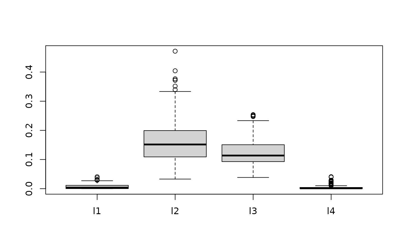
The plot below shows posterior draws of the for the simulated data under the two scenarios allowing different by dimension with and without selection.
boxplot(as.data.frame(fit.bark.d$theta.lambda))
boxplot(as.data.frame(fit.bark.sd$theta.lambda))
While the plots of the without selection (top) and with selection (bottom) are similar, the additional shrinkage of values towards zero has lead to an improvement in RMSE.
Comparison
We will compare {r bark} to two other popular methods, {r BART} and {r SVM} that provide flexible models that are also non-linear in the input variables.
bart.available =  suppressMessages(require(BART))
svm.available  =  suppressMessages(require(e1071))
io.available = suppressMessages(require(fdm2id))BART
if (bart.available) {
 y.loc = match("y", colnames(traindata))
 friedman2.bart = wbart(x.train = as.matrix(traindata[ , -y.loc]),
                        y.train =  traindata$y)
  pred.bart =   predict(friedman2.bart,
                        as.matrix(testdata[ , -y.loc]))
  yhat.bart = apply(pred.bart, 2, mean)
  mean((yhat.bart - testdata$y)^2)
}
#> *****Into main of wbart
#> *****Data:
#> data:n,p,np: 200, 4, 0
#> y1,yn: -160.199247, -161.188667
#> x1,x[n*p]: 91.480604, 2.404099
#> *****Number of Trees: 200
#> *****Number of Cut Points: 100 ... 100
#> *****burn and ndpost: 100, 1000
#> *****Prior:beta,alpha,tau,nu,lambda: 2.000000,0.950000,33.129480,3.000000,7744.575956
#> *****sigma: 199.394818
#> *****w (weights): 1.000000 ... 1.000000
#> *****Dirichlet:sparse,theta,omega,a,b,rho,augment: 0,0,1,0.5,1,4,0
#> *****nkeeptrain,nkeeptest,nkeeptestme,nkeeptreedraws: 1000,1000,1000,1000
#> *****printevery: 100
#> *****skiptr,skipte,skipteme,skiptreedraws: 1,1,1,1
#>
#> MCMC
#> done 0 (out of 1100)
#> done 100 (out of 1100)
#> done 200 (out of 1100)
#> done 300 (out of 1100)
#> done 400 (out of 1100)
#> done 500 (out of 1100)
#> done 600 (out of 1100)
#> done 700 (out of 1100)
#> done 800 (out of 1100)
#> done 900 (out of 1100)
#> done 1000 (out of 1100)
#> time: 2s
#> check counts
#> trcnt,tecnt,temecnt,treedrawscnt: 1000,0,0,1000
#> *****In main of C++ for bart prediction
#> tc (threadcount): 1
#> number of bart draws: 1000
#> number of trees in bart sum: 200
#> number of x columns: 4
#> from x,np,p: 4, 1000
#> ***using serial code
#> [1] 4605.555
Classification Example
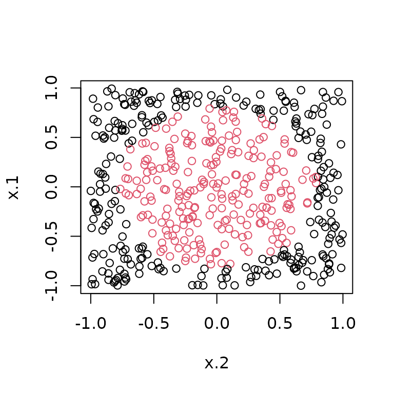
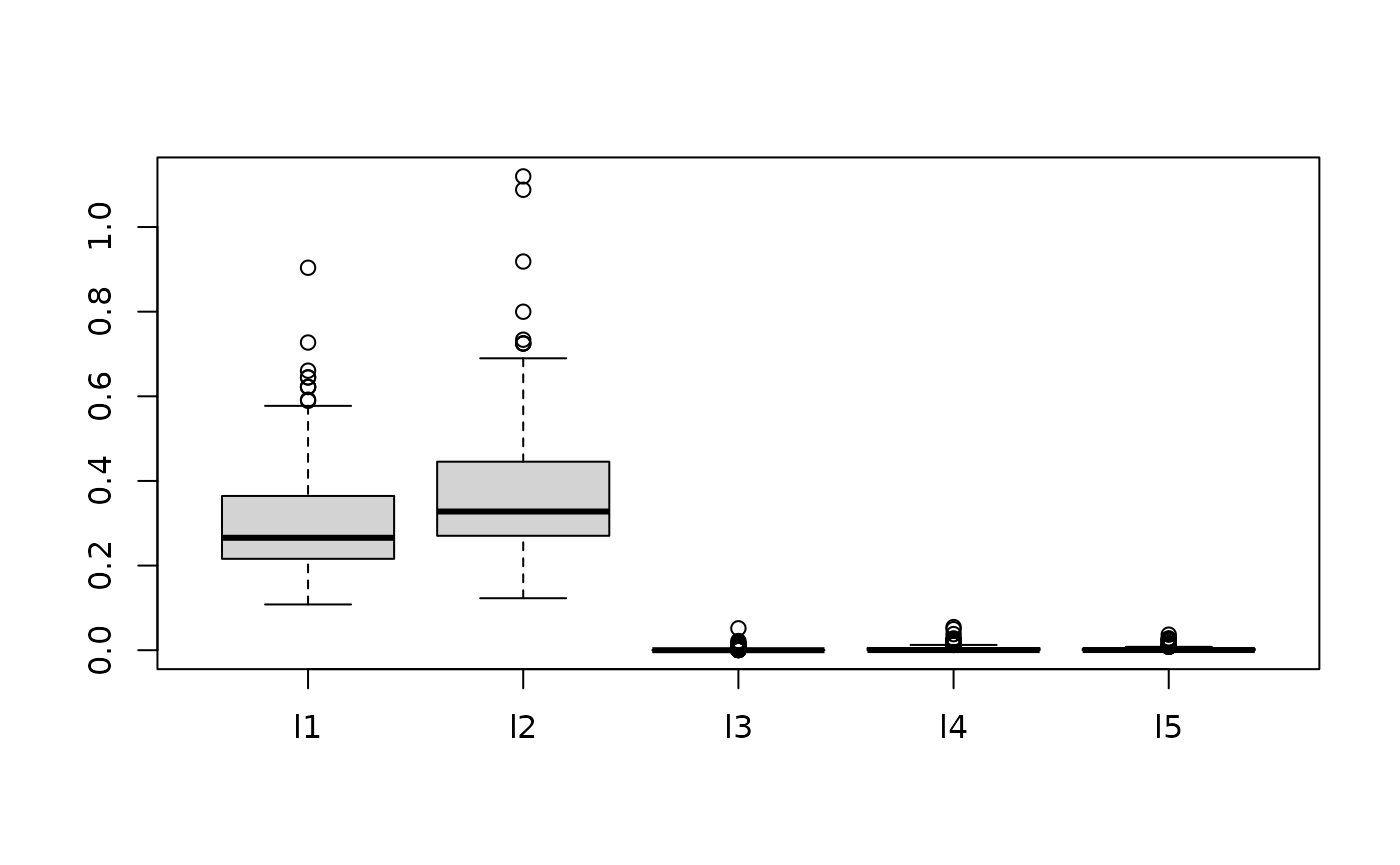
The data are generated so that only the first 2 dimensions matter
set.seed(42)
n = 500
circle2 = data.frame(sim_circle(n, dim = 5))
train = sample(1:n, size = floor(n/2), rep=FALSE)
plot(x.1 ~ x.2, data=circle2, col=y+1)
set.seed(42)
circle2.bark = bark(y ~ ., data=circle2, subset=train,
                    testdata = circle2[-train,],
                    classification = TRUE,
                    selection = TRUE,
                    common_lambdas = FALSE,
                    fixed = list(eps = .5, gam = 5),
                    nburn = 100,
                    nkeep = 250,
                    printevery = 10^10)
#Classify
#
mean((circle2.bark$yhat.test.mean > 0) != circle2[-train, "y"])
#> [1] 0.024
The plot below shows posterior draws of the for the simulated data.
boxplot(as.data.frame(circle2.bark$theta.lambda)) ## SVM
if (svm.available) {
  circle2.svm = svm(y ~ ., data=circle2[train,], type="C")
  pred.svm = predict(circle2.svm, circle2[-train,])
  mean(pred.svm != circle2[-train, "y"])
}
#> [1] 0.104
if (bart.available) {
  y.loc = match("y", colnames(circle2))
  circle.bart = pbart(x.train = as.matrix(circle2[train, -y.loc]),
                            y.train =  circle2[train, y.loc])
  pred.bart =   predict(circle.bart, as.matrix(circle2[-train, -y.loc]))
  mean((pred.bart$prob.test.mean > .5) != circle2[-train, y.loc])
}
#> *****Into main of pbart
#> *****Data:
#> data:n,p,np: 250, 5, 0
#> y1,yn: 0, 0
#> x1,x[n*p]: -0.791174, 0.207159
#> *****Number of Trees: 50
#> *****Number of Cut Points: 100 ... 100
#> *****burn and ndpost: 100, 1000
#> *****Prior:mybeta,alpha,tau: 2.000000,0.950000,0.212132
#> *****binaryOffset: -0.030084
#> *****Dirichlet:sparse,theta,omega,a,b,rho,augment: 0,0,1,0.5,1,5,0
#> *****nkeeptrain,nkeeptest,nkeeptreedraws: 1000,1000,1000
#> *****printevery: 100
#> *****skiptr,skipte,skiptreedraws: 1,1,1
#>
#> MCMC
#> done 0 (out of 1100)
#> done 100 (out of 1100)
#> done 200 (out of 1100)
#> done 300 (out of 1100)
#> done 400 (out of 1100)
#> done 500 (out of 1100)
#> done 600 (out of 1100)
#> done 700 (out of 1100)
#> done 800 (out of 1100)
#> done 900 (out of 1100)
#> done 1000 (out of 1100)
#> time: 1s
#> check counts
#> trcnt,tecnt: 1000,0
#> *****In main of C++ for bart prediction
#> tc (threadcount): 1
#> number of bart draws: 1000
#> number of trees in bart sum: 50
#> number of x columns: 5
#> from x,np,p: 5, 250
#> ***using serial code
#> [1] 0.056